Renaissance Simulations Laboratory
Explore the first galaxies through physics-based modeling, simulation, and data exploration
Learn
This is where you can learn about the first galaxies in the universe, how we can use supercomputers to study them, and what this site enables you to do.
The first galaxies in the universe
Then and now
The universe is filled with countless galaxies today. But there was a time not long after the big bang when there were no galaxies at all—just tiny fluctuations in the density of matter. How does a featureless universe “grow galaxies”? And how do they differ from modern galaxies like the Milky Way? learn more
Growing Galaxies
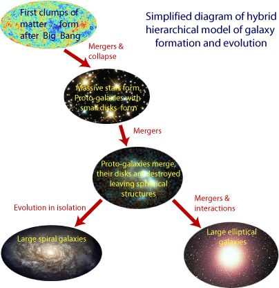
Gravity collects regions of slight overdensity in the early universe into dense clumps of gas and dark matter cosmologists call halos. These halos merge and coalesce to form the first galaxies (protogalaxies). As time goes on, protogalaxies merge and coalesce into larger galaxies, and so on, until today we have a variety of galaxy types and sizes. These include large spiral galaxies like the Milky Way, and large elliptical galaxies, like M87. Thus, galaxies are said to grow hierarchically, with large modern galaxies representing the assembly of thousands of protogalaxies which are much smaller. learn more
Observing the First Galaxies
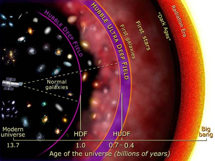
Can we observe the first galaxies directly? No. They are too small and too faint for the Hubble Space Telescope (HST) to detect them. However the HST can detect very faint, distant galaxies which are likely second and third generation galaxies. The graphic at right shows how deep the HST has been able to probe. The Hubble Ultra Deep Field has detected galaxies when the universe was only 6400-700 million years old, which is only a few percent of its present age. The James Webb Space Telescope, to be launched by NASA in 2018, should be able to observe even younger galaxies, pushing into the realm of truly first galaxies. learn more
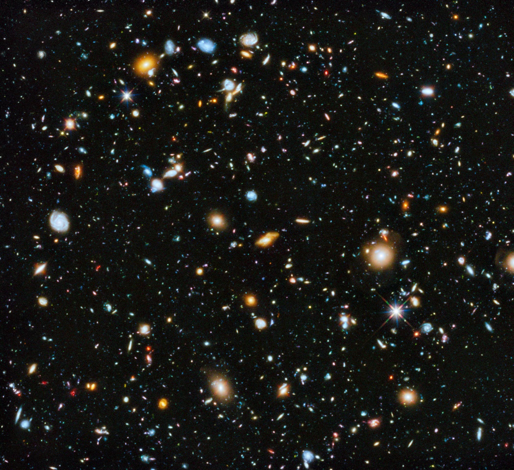
Faint Red Blobs at the Edge of the Universe
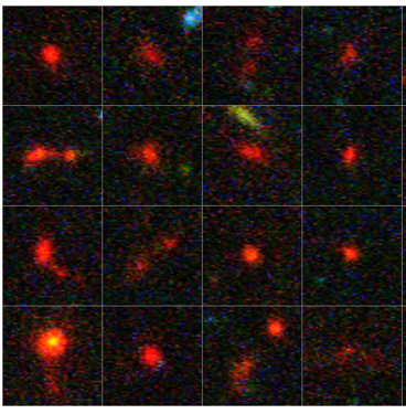
While not strictly the first galaxies in the universe, the most distant galaxies detected by the HST are worthy of study. They appear as faint red blobs in the Hubble Ultra Deep Field. They are red because the expansion of the universe has redshifted their starlight into the red part of the visible spectrum. They are faint because they are distant. And they are very small compared to the Milky Way galaxy. A typical size is about 500 parsec, which is 1/50 the size of the Milky Way galaxy. learn more.
How we use supercomputers to study the first galaxies
Before we delve into how we use supercomputers to study the first galaxies, we need to cover some basics.
Supercomputers
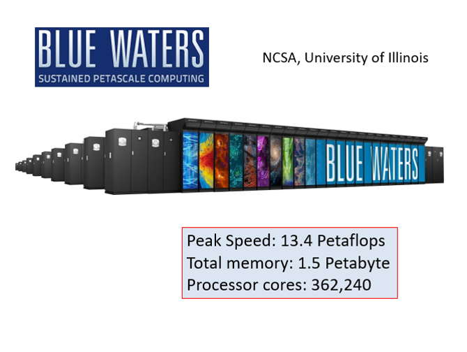
Supercomputers are large clusters of processing “nodes” all connected together by a fast network so that it can act like a single, very powerful computer. Each node can have dozens of processing “cores”. For example, The Blue Waters supercomputer, used for the Renaissance Simulations, has over 22,640 nodes, each with 16 cores, for a total of 362,240 processing elements. learn more
Parallel computing
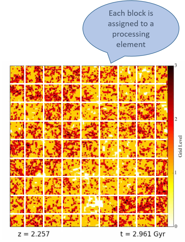
Supercomputers are programmed using a technique called parallel computing. Quite simply, a large problem (like computing the universe) is subdivided into many smaller problems (like compute this piece of the universe), and each smaller problem is assigned to one of the computing cores or nodes. All these smaller problems are computed simultaneously, or “in parallel”, with information about their state being continuously communicated to neighboring processors in order to maintain physical correctness and synchronicity. Typically, the subdivision of the big problem into many smaller problems is done using domain decomposition, illustrated at right. learn more
Coping with an infinite universe
Obviously, we cannot fit an infinite universe into a finite computer, however large and powerful. Instead, we simulate a chunk of the universe that is large enough to have lots of interesting things in it (galaxies, clusters, superclusters, etc.) In practice, we adjust the size of the chunk according to what we are interested in. For example, if we are interested in superclusters, which are far larger than individual galaxies, then we would simulate a larger chunk of the universe than if we were only interested in an individual galaxy. The shape of the chunk is taken to be a cube for computational convenience. We assume period boundary conditions in all three dimensions to mimic the presence of matter outside the box we are simulating.
Coping with an expanding universe
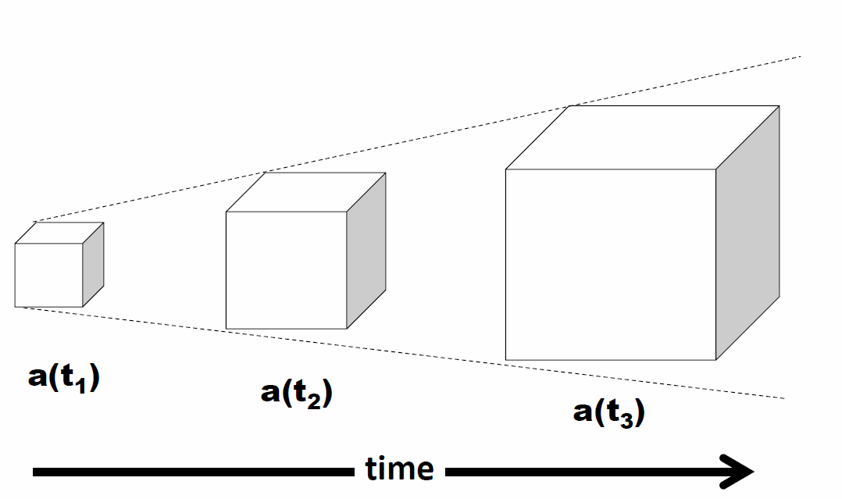
Hubble discovered the universe is expanding in 1929. What that means is that every point in the universe is moving away from every other point in the universe with uniform speed. That speed varies with time, and also depends on how far apart the two points are. While this seems a little boggling, just think about the raisins in a lump of raisin bread dough. As the dough rises, the raisins behave just as described above. But how to simulate a cube of matter embedded in an expanding universe? Easy. We simulate a cube of the universe that expands at exactly the rate of the expanding universe. We say we simulate a co-moving volume of the universe.
Initializing the simulation
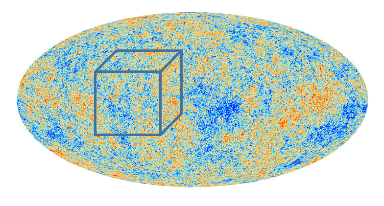
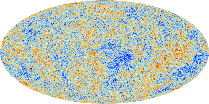
We have already learned that through detailed observations of the cosmic microwave background, we know what the universe was like 380,000 years after the big bang. We use that information to initialize our simulations. Specifically we know that the matter in the universe was very homogenous, with only slight ripples imposed that create regions of slight overdensity and underdensity. We call these matter fluctuations. The amplitude and power spectrum of these matter fluctuations has been precisely measured by the Planck satellite. Generally, we do not start the simulation at t=380,000 yr, but some millions of years later. Using linear perturbation theory, we are able to adjust the amplitude accordingly, however the power spectrum remains the same.
Computing what happens next
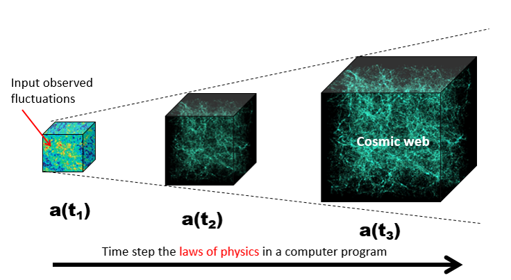
Fortunately, the physical laws that governs what happens next are well understood. We program these physical laws into a parallel computer program, and step the physical state of the universe along in a number of discrete steps, called timesteps. A cosmological simulation can have anywhere from a few thousand timesteps to over 100,000 timesteps, depending on how far into cosmic history you want to simulate, and how finely resolved the simulation is. learn more
What physical laws are programmed?
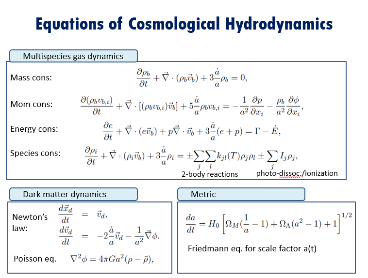
The physical laws are expressed as differential equations, both ordinary and partial, which govern the time evolution of the matter and energy in the simulation. Specifically, the following processes are included:
- Uniform by time-varying expansion of the universe as a whole
- Dynamical behavior of dark matter under the action of self-gravity
- Dynamical, thermodynamical, and ionization behavior of the hydrogen and helium gas left over from the big bang
- Chemistry and radiative cooling of the gas and condensation of stars out of the coldest gas
- Feedback of energy, radiation, and heavy elements from stars
- Feedback of high energy radiation from accreting stellar remnants
- Transport of photoionizing and photodissociating radiation
Ok, so what happens?
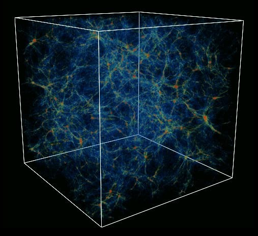
The narrated animation below shows what happens when all this physics is put into a supercomputer, and let loose for hundreds of millions of cosmic years, and millions of computer-hours. First stars form, which explode as supernovae after a few million years, setting the stage for the formation of protogalactic building bocks. They merge due to gravity to form the first galaxies in the universe. Voila!
About the Renaissance Simulations Laboratory (RSL)
Purpose
The RSL is an open data resource where the Renaissance Simulations data can be browsed, accessed, and analyzed. The site supports visual data exploration, data download, as well as interactive analysis through the use of Jupyter notebooks. The site is also a place for sharing your scientific analysis and results.
How to use
The RSL is organized into 4 departments according to your goals:
- LEARN – learn about the first galaxies, how we use supercomputers to understand them, and the purpose and uses for the RSL
- INVESTIGATE – download or analyze the data using the yt tookit in a Jupyter notebook
- SHOWCASE – showcase your results through image galleries, animations, or publications
- USER GUIDE - documentation on available data products and analyzing on the RSL
Acknowledgements
The RSL is partially supported by NSF CDS&E grant 1615848, with additional resources provided by the San Diego Supercomputer Center and the National Center for Supercomputing Applications.